Let  be a compact smooth manifold and
  a transitive Anosov
  diffeomorphism. If
  is an
is an  -invariant Borel probability measure on that is absolutely continuous with respect to volume, then the Hopf argument can be used to show that is ergodic. In fact, recently it has been shown that even stronger ergodic properties such as multiple mixing can be deduced; for example, see Coudène, Hasselblatt, and Troubetzkoy [Stoch. Dyn. 16 (2016), no. 2].
A more general class of measures with strong ergodic properties is given by the theory of thermodynamic formalism developed in the 1970s: given any Hölder continuous potential  , the quantity
  is maximized by a unique invariant Borel probability measure
  , which is called the equilibrium state of
  ; the maximum value of the given quantity is the topological pressure
  . The unique equilibrium state has the Gibbs property: for every
  there is a constant
  such that
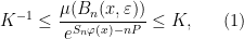
where  is the Bowen ball around
  of order
  and radius
  , and we write
 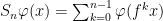 for the th ergodic sum along the orbit of .
Historically, strong ergodic properties (mixing, K, Bernoulli) for equilibrium states have been established using methods such as Markov partitions rather than via the Hopf argument. However, in the more general non-uniformly hyperbolic setting, it can be difficult to extend these symbolic arguments, and so it is interesting to ask whether the Hopf argument can be applied instead, even if it only recovers some of the strong ergodic properties. The key property of absolutely continuous measures that is needed for the Hopf argument is the fact that they have a local product structure, which we define below. It was shown by Haydn [Random Comput. Dynam. 2 (1994), no. 1, 79–96] and by Leplaideur [Trans. Amer. Math. Soc. 352 (2000), no. 4, 1889–1912] that in the uniformly hyperbolic setting, the equilibrium states  have local product structure when is Hölder continuous; thus one could apply the Hopf argument to them.
This post contains a direct proof that any measure with the Gibbs property (1) has local product structure; see Theorem 3 below. (This will be a bit of a longer post, since we need to recall several different concepts and then do some non-trivial technical work.) Since Bowen’s proof of uniqueness of equilibrium states using specification [Math. Systems Theory 8 (1974/1975), no. 3, 193–202] establishes the Gibbs property, this means that the equilibrium states produced this way could be addressed with the Hopf argument (I haven’t carried out the details yet, so I claim no formal results here). I should point out, though, that even without the use of Markov partitions, Ledrappier showed that these measures have the K property, which in particular implies multiple mixing. Since multiple mixing is the strongest thing we might hope to get from the Hopf argument, my primary motivation for the present approach is that Dan Thompson and I recently generalized Bowen’s result to systems satisfying a certain non-uniform specification property [Adv. Math. 303 (2016), 745–799], and the unique equilibrium states we obtain satisfy a non-uniform version of the Gibbs property (1), so it is reasonable to hope that they also have local product structure and can be studied using the Hopf argument; but this is beyond the scope of this post and will be addressed in a later paper.
1. Local product structure
Before defining local product structure for , we recall some definitions. Since is Anosov, every  has local stable and unstable manifolds
  , which have the following properties.
- There are
 and
and  such that for all ,
  , and
, and  , we have
  ; a similar contraction bound holds going backwards in time when
  .
.
- There is
 such that if
  for all , then ; similarly for
  with
with  .
.
- There is such that if
 , then
  is a single point, which we denote
 ![{[x,y]}](https://s0.wp.com/latex.php?latex=%7B%5Bx%2Cy%5D%7D&bg=ffffff&fg=000000&s=0&c=20201002) . Moreover, there is a constant
. Moreover, there is a constant  such that
 ![{d([x,y],x) \leq Q d(x,y)}](https://s0.wp.com/latex.php?latex=%7Bd%28%5Bx%2Cy%5D%2Cx%29+%5Cleq+Q+d%28x%2Cy%29%7D&bg=ffffff&fg=000000&s=0&c=20201002) , and similarly for
, and similarly for ![{d([x,y],y)}](https://s0.wp.com/latex.php?latex=%7Bd%28%5Bx%2Cy%5D%2Cy%29%7D&bg=ffffff&fg=000000&s=0&c=20201002) .
.
A set  is a rectangle if it has diameter
  and is closed under the bracket operation: in other words, for every
  , the intersection point
 ![{[x,y] = W_x^s \cap W_y^u}](https://s0.wp.com/latex.php?latex=%7B%5Bx%2Cy%5D+%3D+W_x%5Es+%5Ccap+W_y%5Eu%7D&bg=ffffff&fg=000000&s=0&c=20201002) exists and is contained in
exists and is contained in  .
.
Lemma 1 For every , there is a rectangle containing .
Proof: Write  and similarly for
  . Consider the set
 ![{R = \{[y,z] : y\in V_x^u, z\in V_x^s\}}](https://s0.wp.com/latex.php?latex=%7BR+%3D+%5C%7B%5By%2Cz%5D+%3A+y%5Cin+V_x%5Eu%2C+z%5Cin+V_x%5Es%5C%7D%7D&bg=ffffff&fg=000000&s=0&c=20201002) and observe that for every
and observe that for every ![{[y,z]\in R}](https://s0.wp.com/latex.php?latex=%7B%5By%2Cz%5D%5Cin+R%7D&bg=ffffff&fg=000000&s=0&c=20201002) we have
we have
![\displaystyle d([y,z],x) \leq d([y,z],y) + d(y,x) \leq (Q+1)d(y,x) \leq \tfrac\varepsilon2.](https://s0.wp.com/latex.php?latex=%5Cdisplaystyle++d%28%5By%2Cz%5D%2Cx%29+%5Cleq+d%28%5By%2Cz%5D%2Cy%29+%2B+d%28y%2Cx%29+%5Cleq+%28Q%2B1%29d%28y%2Cx%29+%5Cleq+%5Ctfrac%5Cvarepsilon2.+&bg=ffffff&fg=000000&s=0&c=20201002)
Thus has diameter  , and for every
 ![{[y,z], [y',z']\in R}](https://s0.wp.com/latex.php?latex=%7B%5By%2Cz%5D%2C+%5By%27%2Cz%27%5D%5Cin+R%7D&bg=ffffff&fg=000000&s=0&c=20201002) we have
we have
![\displaystyle [[y,z],[y',z']] = W_{[y,z]}^s \cap W_{[y',z']}^u = W^s_y \cap W^u_{z'} = [y,z'] \in R,](https://s0.wp.com/latex.php?latex=%5Cdisplaystyle++%5B%5By%2Cz%5D%2C%5By%27%2Cz%27%5D%5D+%3D+W_%7B%5By%2Cz%5D%7D%5Es+%5Ccap+W_%7B%5By%27%2Cz%27%5D%7D%5Eu+%3D+W%5Es_y+%5Ccap+W%5Eu_%7Bz%27%7D+%3D+%5By%2Cz%27%5D+%5Cin+R%2C+&bg=ffffff&fg=000000&s=0&c=20201002)
so is indeed a rectangle. 
Given and a rectangle  , let
, let  . Then can be recovered from
  via the method in the proof above, as the image of the map
 ![{[\cdot,\cdot] \colon V_x^u \times V_x^s \rightarrow M}](https://s0.wp.com/latex.php?latex=%7B%5B%5Ccdot%2C%5Ccdot%5D+%5Ccolon+V_x%5Eu+%5Ctimes+V_x%5Es+%5Crightarrow+M%7D&bg=ffffff&fg=000000&s=0&c=20201002) . Given measures
. Given measures  on , let
  be the pushforward of
  under this map; that is, for every pair of Borel sets
  and
and  , we put
 ![{(\nu^u\otimes \nu^s)(\{[y,z] : y\in A, z\in B\}) = \nu^u(A)\nu^s(B)}](https://s0.wp.com/latex.php?latex=%7B%28%5Cnu%5Eu%5Cotimes+%5Cnu%5Es%29%28%5C%7B%5By%2Cz%5D+%3A+y%5Cin+A%2C+z%5Cin+B%5C%7D%29+%3D+%5Cnu%5Eu%28A%29%5Cnu%5Es%28B%29%7D&bg=ffffff&fg=000000&s=0&c=20201002) .
.
Definition 2 A measure has local product structure with respect to  if for every and rectangle there are measures on such that
 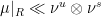 .
.
Theorem 3 Let be a  Anosov diffeomorphism,
  a Hölder continuous function, and an -invariant Borel probability measure on satisfying the Gibbs property (1) for some
  . Then has local product structure in the sense of Definition 2. Moreover, there is
  such that for all , the measures can be chosen so that the Radon–Nikodym derivative
  satisfies
  at -a.e. point.
A quick side remark: here the diffeomorphism is only required to be . The reason for the hypothesis at the beginning of this post was so that the geometric potential  is Hölder continuous and its unique equilibrium state (the absolutely continuous invariant measure if it exists, or more generally the SRB measure) has the Gibbs property; this may not be true if is only .
2. Conditional measures
In order to prove Theorem 3, we must start by recalling the notion of conditional measures; see Coudène’s book (especially Chapters 14 and 15) or Viana’s notes for more details than what is provided here.
Let  be a Lebesgue space. A partition of
  is a map
  such that for -a.e.
  , the sets
  and
and  either coincide or are disjoint. Write
  for the set of partition elements, and say that the partition
  is finite if
  is finite.
Given a finite partition , it is easy to define conditional measures  on the set for -a.e. by writing
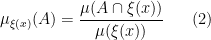
when  , and ignoring those partition elements with zero measure. One can recover the measure from its conditional measures by the formula

If we write  for the measure on defined by putting
  for all
  , then (3) can be written as
Even when the partition is infinite, one may still hope to obtain a formula along the lines of (4).
Example 1 Let be the unit square, be two-dimensional Lebesgue measure, and be the horizontal line through . Then Fubini’s theorem gives (4) by taking  to be Lebesgue measure on horizontal lines, and defining on , the set of horizontal lines in
 ![{[0,1]^2}](https://s0.wp.com/latex.php?latex=%7B%5B0%2C1%5D%5E2%7D&bg=ffffff&fg=000000&s=0&c=20201002) , in one of the two following (equivalent) ways:
, in one of the two following (equivalent) ways:
- given
 , let
, let  ;
;
- identify with the interval
![{\{0\}\times [0,1]}](https://s0.wp.com/latex.php?latex=%7B%5C%7B0%5C%7D%5Ctimes+%5B0%2C1%5D%7D&bg=ffffff&fg=000000&s=0&c=20201002) on the
on the  -axis, and define as the image of one-dimensional Lebesgue measure on this interval.
Note that must satisfy the first of these no matter what the partition is, while the second is a convenient description of in this particular example.
A similar-looking example (and the one which is most relevant for our purposes) comes by letting be a rectangle and letting  be the partition into local unstable leaves. To produce conditional measures
  , we need to use the fact that the partition is measurable. This means that there is a sequence of finite partitions
  that refines to in the sense that for -a.e. , we have

Lemma 4 Given any rectangle , the partition of into local unstable leaves is measurable.
Proof: Fix  and let
  be a refining sequence of finite partitions of
  with the property that
  for all
  ; then let
  , and we are done.
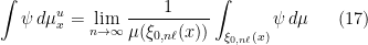
Whenever is a measurable partition of a compact metric space , we can define the conditional measures  as the limits of the conditional measures
  . Indeed, one can show (we omit the proofs) that for -a.e. , the limit
  exists for every continuous
  and defines a continuous linear functional
  ; the corresponding measures satisfy

for every  , where once again we put .
The key result that we will need to describe properties of  when is the partition of into local unstable leaves is that for -a.e.
  and every , we have

where is any sequence of finite partitions that refines to .
In order to establish the local product structure for that is claimed by Theorem 3, we will show that the measures vary in an absolutely continuous manner as varies within . That is, we consider for every the holonomy map  defined by moving along local stable manifolds, so
![\displaystyle \pi_{x,y}(z) = [z,y] = V_z^s \cap V_{y}^u \text{ for all } z\in V_x^u.](https://s0.wp.com/latex.php?latex=%5Cdisplaystyle++%5Cpi_%7Bx%2Cy%7D%28z%29+%3D+%5Bz%2Cy%5D+%3D+V_z%5Es+%5Ccap+V_%7By%7D%5Eu+%5Ctext%7B+for+all+%7D+z%5Cin+V_x%5Eu.+&bg=ffffff&fg=000000&s=0&c=20201002)
Our goal is to use the Gibbs property (1) for to prove that for every rectangle and -a.e. , the conditional measures  and
and  satisfy

Once this is established, we can proceed as follows. Consider a rectangle with the decomposition into local unstable manifolds, let be such that (7) holds for -a.e. , and then identify with , as in the second characterization of in Example 1. Let  be the measure on corresponding to under this identification, and let
  . Given , let
 ![{\psi_y = \frac{d(\pi_{x,y})_* \mu_x^u}{d\mu_{y}^u} \colon V_y^u \rightarrow [\bar{K}^{-1},\bar{K}]}](https://s0.wp.com/latex.php?latex=%7B%5Cpsi_y+%3D+%5Cfrac%7Bd%28%5Cpi_%7Bx%2Cy%7D%29_%2A+%5Cmu_x%5Eu%7D%7Bd%5Cmu_%7By%7D%5Eu%7D+%5Ccolon+V_y%5Eu+%5Crightarrow+%5B%5Cbar%7BK%7D%5E%7B-1%7D%2C%5Cbar%7BK%7D%5D%7D&bg=ffffff&fg=000000&s=0&c=20201002) , so that in particular we have
, so that in particular we have
![\displaystyle \int_{V_y^u} \varphi\,d\mu_y^u = \int_{V_y^u} \frac{\varphi}{\psi_y}\, d(\pi_{x,y})_*\mu_x^u = \int_{V_x^u} \frac{\varphi([z,y])}{\psi_y([z,y])} \,d\mu_x^u](https://s0.wp.com/latex.php?latex=%5Cdisplaystyle++%5Cint_%7BV_y%5Eu%7D+%5Cvarphi%5C%2Cd%5Cmu_y%5Eu+%3D+%5Cint_%7BV_y%5Eu%7D+%5Cfrac%7B%5Cvarphi%7D%7B%5Cpsi_y%7D%5C%2C+d%28%5Cpi_%7Bx%2Cy%7D%29_%2A%5Cmu_x%5Eu+%3D+%5Cint_%7BV_x%5Eu%7D+%5Cfrac%7B%5Cvarphi%28%5Bz%2Cy%5D%29%7D%7B%5Cpsi_y%28%5Bz%2Cy%5D%29%7D+%5C%2Cd%5Cmu_x%5Eu+&bg=ffffff&fg=000000&s=0&c=20201002)
for every continuous  . Then by (5), we have
![\displaystyle \begin{aligned} \int\varphi\,d\mu &= \int_{\Xi} \int_C \varphi \,d\mu_C \,d\hat\mu(C) = \int_{V_x^s} \int_{V_y^u} \varphi \,d\mu_y^u \,d\nu^s(y) \\ &= \int_{V_x^s} \int_{V_x^u} \frac{\varphi([z,y])}{\psi_y([z,y])} \,d\nu^u(z) \,d\nu^s(y). \end{aligned}](https://s0.wp.com/latex.php?latex=%5Cdisplaystyle++%5Cbegin%7Baligned%7D+%5Cint%5Cvarphi%5C%2Cd%5Cmu+%26%3D+%5Cint_%7B%5CXi%7D+%5Cint_C+%5Cvarphi+%5C%2Cd%5Cmu_C+%5C%2Cd%5Chat%5Cmu%28C%29+%3D+%5Cint_%7BV_x%5Es%7D+%5Cint_%7BV_y%5Eu%7D+%5Cvarphi+%5C%2Cd%5Cmu_y%5Eu+%5C%2Cd%5Cnu%5Es%28y%29+%5C%5C+%26%3D+%5Cint_%7BV_x%5Es%7D+%5Cint_%7BV_x%5Eu%7D+%5Cfrac%7B%5Cvarphi%28%5Bz%2Cy%5D%29%7D%7B%5Cpsi_y%28%5Bz%2Cy%5D%29%7D+%5C%2Cd%5Cnu%5Eu%28z%29+%5C%2Cd%5Cnu%5Es%28y%29.+%5Cend%7Baligned%7D+&bg=ffffff&fg=000000&s=0&c=20201002)
By Definition 2, this shows that has local product structure with respect to . Thus in order to prove Theorem 3, it suffices to shows that Gibbs measures satisfy the absolute continuity property (7).
It is worth noting quickly that our use of the term “absolute continuity” here has a rather different meaning from another common concept, which is that of a measure with “absolutely continuous conditional measures on unstable manifolds”. This latter notion is essential for the definition of SRB measures (indeed, in the Anosov setting it is the definition), and involves comparing to volume measure on , instead of to the pushforwards of other conditional measures under holonomy.
3. Adapted partitions
In order to prove the absolute continuity property (7), we need to obtain estimates on . We start by getting estimates on from the Gibbs property (1), and then using these to get estimates on using (6).
We will need a family of partitions of that refines to the partition into points. Fix a reference point  , and suppose we have chosen partitions
  of
of  and
and  of
of  for
for  . Then we can define a partition
  of by taking the direct product of these two partitions, using the foliations of by local stable and unstable leaves: that is, we put
![\displaystyle \xi_{m,n}(y) = \{z\in R : \eta_m^u([z,q]) = \eta_m^u([y,q]) \text{ and } \eta_n^s([q,z]) = \eta_n^s([q,y]) \} \ \ \ \ \ (8)](https://s0.wp.com/latex.php?latex=%5Cdisplaystyle++%5Cxi_%7Bm%2Cn%7D%28y%29+%3D+%5C%7Bz%5Cin+R+%3A+%5Ceta_m%5Eu%28%5Bz%2Cq%5D%29+%3D+%5Ceta_m%5Eu%28%5By%2Cq%5D%29+%5Ctext%7B+and+%7D+%5Ceta_n%5Es%28%5Bq%2Cz%5D%29+%3D+%5Ceta_n%5Es%28%5Bq%2Cy%5D%29+%5C%7D+%5C+%5C+%5C+%5C+%5C+%288%29&bg=ffffff&fg=000000&s=0&c=20201002)
In order to obtain information on  using the Gibbs property (1), we need to put an extra condition on the partitions we use; we need to them to be adapted, meaning that each partition element both contains a Bowen ball and is contained within a larger Bowen ball. Most of the ideas here are fairly standard in thermodynamic formalism, but it is important for us to work separately on the stable and unstable manifolds, then combine the two, so we describe things explicitly. Fix . Given
  and
and  , let
, let

Similarly, given  and , let
Given  , we say that the partitions are -adapted if for every partition element
  there is such that

We make a similar definition for using  . Note that we can produce an -adapted sequence of partitions as follows:
- say that
 is
is  -separated if for every
  there is
  such that
  ;
;
- let
 be a maximal -separated set and observe that
  , while the sets
  are disjoint;
- enumerate
 as
as  , and build an -adapted partition by considering the sets
Lemma 5 Let be a measure satisfying the Gibbs property (1). Then there are and  such that if and are -adapted partitions of and , then the product partition defined in (8) satisfies

for every .
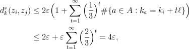
Proof: First we show that the upper bound in (10) holds whenever is sufficiently small. Fix  such that the Gibbs bound (1) holds for Bowen balls of radius
  , and such that
  is significantly smaller than the size of any local stable or unstable leaf. It suffices to show that for every we have
  for some , since then (1) gives the upper bound, possibly with a different constant; note that replacing with in the denominator changes the quantity by at most a constant factor, using the fact that is Hölder continuous together with some basic properties of Anosov maps. (See, for example, Section 2 of this previous post for a proof of this Bowen property.)
Given  such that and lie on the same local stable leaf with
  , let
, let

be the closest that any holonomy along local unstable leaves can bring and . Note that  is positive and continuous in and ; by compactness there is
  such that
  for all
  as above. In particular, this means that if are the images under an (unstable) holonomy of some
  with
with  , then we must have
  .
.
Choose  similarly for stable holonomies, and fix
  . Fix , ,
  , and
, and  . Then for every
  we have
![\displaystyle d(f^k[y',z'],f^k[y,z]) \leq d(f^k[y',z'],f^k[y',z]) + d(f^k[y',z],f^k[y,z]). \ \ \ \ \ (11)](https://s0.wp.com/latex.php?latex=%5Cdisplaystyle++d%28f%5Ek%5By%27%2Cz%27%5D%2Cf%5Ek%5By%2Cz%5D%29+%5Cleq+d%28f%5Ek%5By%27%2Cz%27%5D%2Cf%5Ek%5By%27%2Cz%5D%29+%2B+d%28f%5Ek%5By%27%2Cz%5D%2Cf%5Ek%5By%2Cz%5D%29.+%5C+%5C+%5C+%5C+%5C+%2811%29&bg=ffffff&fg=000000&s=0&c=20201002)
These distances can be estimated by observing that ![{f^k[y',z']}](https://s0.wp.com/latex.php?latex=%7Bf%5Ek%5By%27%2Cz%27%5D%7D&bg=ffffff&fg=000000&s=0&c=20201002) and
and ![{f^k[y',z]}](https://s0.wp.com/latex.php?latex=%7Bf%5Ek%5By%27%2Cz%5D%7D&bg=ffffff&fg=000000&s=0&c=20201002) are the images of
are the images of  and
and  under a holonomy map along local unstables, and similarly and
 ![{f^k[y,z]}](https://s0.wp.com/latex.php?latex=%7Bf%5Ek%5By%2Cz%5D%7D&bg=ffffff&fg=000000&s=0&c=20201002) are images of and
are images of and  under a holonomy map along local stables. Then our choice of shows that both quantities in the right-hand side of (11) are
  , which gives the inclusion we needed. This proves the upper bound in (10); the proof of the lower bound is similar.
4. A refining sequence of adapted partitions
Armed with the formula from Lemma 5, we may look at the characterization of conditional measures in (6) and try to prove that the absolute continuity bound (7) holds whenever both satisfy (6). There is one problem before we do this, though; the formula in (6) requires that the sequence of partitions be refining, and there is no a priori reason to expect that the adapted partitions produced by the simple argument before Lemma 5 refine each other. To get this additional property, we must do some more work. To the best of my knowledge, the arguments here are new.
4.1. Strategy
Start by letting  be a maximal
  -separated set. We want to build a refining sequence of adapted partitions using the sets
  , where instead of using Bowen balls with radius
  and we will use Bowen balls with radius and
  ; this does not change anything essential about the previous section. We cannot immediately proceed as in the argument before Lemma 5, because if we are not careful when choosing the elements of the partition , their boundaries might cut the Bowen balls
  for
for  and
and  , spoiling our attempt to build an adapted partition
  that refines .
A first step will be to only build for some values of . More precisely, we fix  such that
  , so that for every and
  , we have
  ; then writing

we have the following for every  :
:

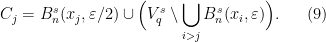
We will only build adapted partitions for those that are multiples of  . We need to understand when the Bowen balls associated to points in the sets can overlap. We write
  .
.
Definition 6 An -path between  and
and  is a sequence
  with
with  and
and  such that
  for all
  . A subset
  is -connected if there is an -path between any two elements of
  .
.
Given  , let
, let  . In the next section we will prove the following.
Proposition 7 If  is -connected and
  , then

For now we show how to build a refining sequence of adapted partitions assuming (14) by modifying the construction in (9). The key is that we build our partitions so that for every -connected , the set  is completely contained in a single element of .
Suppose we have built a partition  with this property; we need to construct a partition that refines , still has this property, and also has the property that every partition element
  has some such that
  . To this end, let
  be an element of the partition , and enumerate the -connected components of
  as
as  , where each
  contains some
  , while each
  is in fact a subset of
  .
.
It follows from (14) that  for all
  . Given
  , we can observe that
  for some
  with
with  . Moreover, the sets
 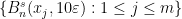 cover , so every
  must intersect some set
  , and hence be contained in some
  . Given , let
  . Then for each , let
  . Define sets
  by
by
It is not hard to verify that the sets  form a partition of such that
  , and such that every -connected component of that has
  is completely contained in some . Repeating this procedure for the other elements of produces the desired .
4.2. Proof of the proposition
Now we must prove Proposition 7. Let  be as in the previous section, so that in particular, every has that is a multiple of , and given any
  we have
  .
.
The following concept is essential for our proof.
Definition 8 Given an -path  , a ford is a pair
  for all
  . Think of “fording a river'' to get from
  to
to  by going through deeper levels of the -path; the alternative is that
  for some , in which case
  is a sort of “bridge'' between
  and
and  .
.
Lemma 9 Suppose that is an -path without any fords, and that  for all
  . Then
  .
.
Proof: By the definition of -path, for every  there is a point
  . Thus

where the second inequality uses (13). Now we need to estimate how often different values of  can appear. Let
  ; we claim that for every
  , we have

First note that  for all
  , because otherwise
  would be a ford. Since the -path has no fords, every
  with
with  must be separated by some
  with
with  , and we conclude that for every , we have

For  , this establishes (16) immediately. If (16) holds up to
  , then this gives

which proves (16) for all by induction. Combining (15) and (16), we have
which proves Lemma 9.
Now we show that the  -separation condition rules out the existence of fords entirely.
Lemma 10 If is an -path, then it has no fords.
Proof: Fix an -path  . Denote the set of fords by

our goal is to prove that  is empty. Put a partial ordering on by writing
![\displaystyle (i',j') \preceq (i,j)\ \Leftrightarrow\ [i',j'] \subset [i,j] \ \Leftrightarrow\ i \leq i' < j' \leq j.](https://s0.wp.com/latex.php?latex=%5Cdisplaystyle++%28i%27%2Cj%27%29+%5Cpreceq+%28i%2Cj%29%5C+%5CLeftrightarrow%5C+%5Bi%27%2Cj%27%5D+%5Csubset+%5Bi%2Cj%5D+%5C+%5CLeftrightarrow%5C+i+%5Cleq+i%27+%3C+j%27+%5Cleq+j.+&bg=ffffff&fg=000000&s=0&c=20201002)
If is non-empty, then since it is finite it must contain some element  that is minimal with respect to this partial ordering. In particular, the -path
  contains no fords, and so by Lemma 9 we have
  , contradicting the assumption that
  (since
  is
is  -separated), and we conclude that must be empty, proving the lemma.
Now we prove Proposition 7. Let be -connected and fix  . Given any
  , there is an -path such that and
  . By Lemma 10, this path has no fords, and so Lemma 9 gives
  . We conclude that
 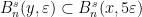 , which proves Proposition 7.
5. Completion of the proof
Thanks to the previous section, we can let and be -adapted partitions of and such that refines whenever  and
and  are both multiples of . By Lemma 5, we have good lower and upper estimates on
  for all , where is the product partition defined in (8). By (6), there is
  with
with  such that for every
  , we have
for every continuous  . The next step towards proving Theorem 3 is the following result.
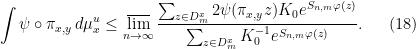
Proposition 11 There is a constant  such that for any
  and every continuous
  , we have
  , where
  is the holonomy map along local unstables.
Proof: Start by fixing for each  a set
a set  such that every element of
  contains exactly one point in
  . Then let
  for every .
Given a positive continuous function  , there is such that if
  , then
  . Thus for all sufficiently large
  , we have whenever
  . For any such and any , we conclude that

where we write 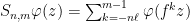 and where the last inequality uses Lemma 5. Similarly,

and we conclude from (6) that
Note that since is Hölder continuous, there are  and
and  such that
  for all
  . Thus given any
  and any , we have

Thus (18) gives
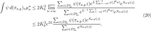
A similar set of computations for shows that

Since  , we can rewrite the sums over
  as sums over
  ; for example,
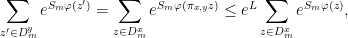
where the inequality uses the fact that the estimate (19) also holds for forward ergodic averages of two points on the same local stable manifold. Using a similar estimate for the numerator in (21) gives
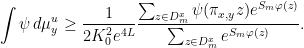
Together with (20), this gives

which completes the proof of Proposition 11.
To complete the proof of Theorem 3, we first observe that for every open set  , there is a sequence of continuous functions
 ![{\psi_n\colon V_y^u \rightarrow (0,1]}](https://s0.wp.com/latex.php?latex=%7B%5Cpsi_n%5Ccolon+V_y%5Eu+%5Crightarrow+%280%2C1%5D%7D&bg=ffffff&fg=000000&s=0&c=20201002) that converge pointwise to the indicator function
that converge pointwise to the indicator function  ; applying Proposition 11 to these functions and using the dominated convergence theorem gives
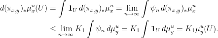
Then for every measurable  , we have
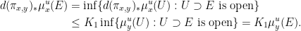
This proves that  and that the Radon–Nikodym derivative is
  -a.e. The lower bound
  follows since the argument is symmetric in and . This proves (7) and thus completes the proof of Theorem 3.

