Our seminar series is taking a hiatus from spectral methods for a couple weeks — these will return eventually, but in the meantime we’ll spend some time with the idea of coupling as a method for deriving statistical properties. In this week’s post, based on Matt Nicol’s talk, we discuss Markov chains and the idea of mixing times.
1. Markov chains and probability distributions
For our purposes, a Markov chain is a (finite or countable) collection of states  and transition probabilities
  , where
  . We write
 ![{P = [p_{ij}]}](https://s0.wp.com/latex.php?latex=%7BP+%3D+%5Bp_%7Bij%7D%5D%7D&bg=ffffff&fg=000000&s=0&c=20201002) for the matrix of transition probabilities. Elements of can be interpreted as various possible states of whatever system we are interested in studying, and represents the probability that the system is in state
for the matrix of transition probabilities. Elements of can be interpreted as various possible states of whatever system we are interested in studying, and represents the probability that the system is in state  at time
  , if it is state
  at time
  . We will think of a Markov chain as a stochastic process with state space
  , representing all sequences
  , where
  is the state of the system at time . The characterisation just given of the transition probabilities can be expressed as

where  represents conditional probability. It is a key feature of a Markov chain (as opposed to other kinds of stochastic processes) that once is known,
  is completely independent of any information on what happened before time — that is, conditioning the probability in (1) on any events involving
  does not change its value.
It is tempting to phrase the above property as “ depends only on ”. However, this formulation is a little misleading, as it gives the impression that the sequence  evolves deterministically, whereas it is of course a stochastic process. To make a correct statement along these lines, we must say that “the probability distribution of depends only on the probability distribution of ”.
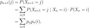
Let us expand this idea. If we write  for the probability that the system is in state at time , then
 ![{p_n\colon S\rightarrow [0,1]}](https://s0.wp.com/latex.php?latex=%7Bp_n%5Ccolon+S%5Crightarrow+%5B0%2C1%5D%7D&bg=ffffff&fg=000000&s=0&c=20201002) has the property that
has the property that 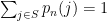 . That is,
  is an element of the unit simplex in
  (if has
  elements) or in
  (if is countably infinite). Write
  for this unit simplex: then the sequence of probability distributions can be viewed as a sequence of points in .
Now the Markov property — the fact that the probability in (1) does not change if we condition on  for
for  — can be reformulated as the property that
  depends only on
  , and not on
  for any . In particular, the Markov chain can be viewed as a (deterministic!) map
  , so once we specify the initial probability distribution
  , subsequent distributions are determined by
  . Our goal will be to understand how the distributions evolve in time — that is, what are the dynamics of the map
  .
.
The map is determined by the transition probabilities (and vice versa). In fact, it can be written in terms of the matrix  using the fact that
so that using the language of matrix multiplication we have

where  represents an arbitrary distribution in . We conclude that iterates of the map correspond to powers of the matrix .
2. Stationary distribution(s)
It is natural to ask if there is a stationary distribution — that is, a distribution  such that if we start the Markov chain in this distribution and then run it forward in time, we keep the same distribution, so that
  for every
  and
and  . If the chain is in such a distribution, then we have a prediction of the long-term behaviour — at any time , no matter how far in the future, we know how likely it is to find the system in a given state.
A related question is to ask about the long-term behaviour when the initial distribution is not stationary. If we start the chain in a distribution such that  , and the probabilities really are changing in time, what happens to as grows? Does the probability of finding the system in state at some later time depend critically on just when we decide to make our observation? Or does converge to some asymptotic probability?
We will answer the first question (existence of stationary distributions) in this section, and address the second later on.
A distribution is stationary for the Markov chain if and only if  — that is, is a fixed point for . In any convex space (such as ), there is a method for looking for fixed points: begin with any distribution , and then consider the Cèsaro averages
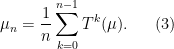
It is not difficult to show that any limit point of this sequence is a fixed point for — that is,  if
if 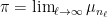 for some
  .
.
To prove this one first needs to clarify what notion of convergence is being used. Consider for now the case when is finite, say  . In this case
  and we can use the usual topology from , so that in particular the simplex is compact and the sequence
  has a convergent subsequence
  . It is a worthwhile exercise to check that the limit
  is in fact a fixed point,
  .
.
Thus we have existence of a stationary distribution when is finite. There are several natural questions to ask at this point, and we address each in turn.
- Is the stationary distribution unique? Or can there be multiple stationary distributions?
- What happens when is countably infinite? Is there a stationary distribution? Is it unique?
- If the stationary distribution
 is unique, then the averaged distributions from (3) converge to . What about the distributions
  themselves, which are just the observations made at time
  , without averaging over ? Do these converge to ?
The answers to these questions are as follows: definitions of the relevant terms will come in a moment.
- The stationary distribution is unique if the Markov chain is irreducible.
- If is countably infinite then there is a stationary distribution if and only if the Markov chain is positive recurrent. If in addition the Markov chain is irreducible then this stationary distribution is unique. For null recurrent and transient chains, there is no stationary distribution.
- If the Markov chain is aperiodic, then the distributions converge to for every initial distribution .
3. Irreducibility
One can associate a directed graph  to a Markov chain by taking for the set of vertices and drawing an edge from to if and only if the transition probability is non-zero.
Now the Markov chain can be interpreted as a random walk on the graph . If at time the random walker is at the vertex labeled , then the probability that he walks to vertex at time is given by the transition probability .
Definition 1 The Markov chain is irreducible if its associated graph is strongly connected — that is, there is a path from any vertex to any other vertex.
The path in Definition 1 may be of any length: an equivalent formulation is that the Markov chain is irreducible if and only if for every there exists such that  .
.
Theorem 2 If is finite and the Markov chain is irreducible, then there is a unique stationary distribution on .
Theorem 2 is part of the Perron–Frobenius theorem in linear algebra.
4. An example — card shuffling
Consider a deck of cards, and let be the set of all possible orderings of those cards, so that  . The act of shuffling the deck can be described as a Markov chain with state space : if
  represents the current order of the cards, then the acts of shuffling once changes the order to some other element of , and the probability of transitioning from the ordering to the ordering encodes some properties of the method of shuffling employed.
One of the simplest possible shuffles is the top-down shuffle — given a deck in state , choose a card at random, remove it from the deck, and place it on the top. Thus there are possible states that can be reached in a single step from the current state, and each one is equally likely. In terms of the random walk on a graph described in the previous section, we have a directed graph with  vertices, each with outgoing degree , and the random walker selects one of the outgoing edges uniformly at random at each step.
It is easy to see that this Markov chain is irreducible — given any two states it is possible to go from one to the other (in enough steps) with positive probability. So there is a unique stationary distribution. What is it? Intuitively we feel as though the shuffling process is symmetric enough (blind enough to the details of the arrangement at any given time) that all arrangements of the cards should be equally likely. In other words, we expect that the stationary distribution is the  defined by
  for all — that is,
  for all .
To see that this distribution is stationary, define for each the set  of configurations of the deck from which the configuration can be reached with a single step of the shuffle (a single selection of a card). Observe that
  has exactly elements, corresponding to the positions in the deck from which the top card in configuration could have been prior to the last shuffle. Thus every vertex in the graph has the same incoming degree , and we can compute
  as
as
Thus is indeed the unique stationary distribution.
Remark 1 The result that every vertex has the same incoming degree can also be derived more abstractly as a consequence of the fact that the symmetric group on elements acts transitively on the graph .
It is natural to ask how many times we must shuffle in order to feel confident that the resulting distribution is “random enough”. In terms of the random walk on the graph , the act of shuffling looks like this: we start with a probability distribution concentrated on a single vertex , corresponding to the initial ordering of the cards. After a single shuffle, that distribution is evenly distributed over the vertices that can be reached from in a single step. After a second shuffle, it is evenly distributed over the  vertices that can be reached from in two steps — except that it is not quite an even distribution now, because some vertices can be reached in multiple ways via a path of length two. For example, itself can be reached in two ways (select the top card twice, or select the second card from the top twice).
As the number of shuffles increases, the distribution gets spread out over more and more vertices, but there is also this phenomenon of recurrence where it comes back to certain vertices more quickly than to others, and does not spread out completely evenly. We would like to understand if it eventually approaches the stationary distribution , which is the uniform distribution on , and if so, how quickly it does so. We will return to this below.
5. Recurrence and transience
When the set of states is infinite, the simplex  is no longer compact, and so the sequence in (3) does not necessarily have a convergent subsequence. In particular, the proof of existence for a stationary distribution given above does not immediately go through.
Indeed, consider the Markov chain with state space  and transition probabilities
  (otherwise). Then the walk is not so random — the walker simply goes from state to state
  at each time step, and in particular we have
  , so
, so  for every , and we see that the distributions converge pointwise to the zero distribution. This is not a probability distribution (the total mass is 0, not 1), and informally we may say that the missing mass has escaped to infinity.
So we need something to replace compactness of , something that will guarantee that no mass escapes to infinity. We may think of this in the language of the previous post — how do we gaurantee precompactness of the sequence ? What conditions on a subset of guarantee that it is precompact?
First we note that because we are now in , not , the notion of convergence and of metric have changed. The relevant metric in this case is the metric

It is helpful to interpret this metric in light of the fact that  are to be thought of as probability distributions. Upon restriction to , the metric (4) (or rather,
  this metric) becomes the total variation metric on the space of probability measures:

where we will prove momentarily that the last three expressions are equivalent. First note that  for all
  . Moreover, if
  are random variables on distributed according to
  respectively, then
and once again the supremum is unchanged if we remove the absolute value signs, as we now see.
Proposition 3 The quantities in (5) all coincide.
Proof: To see that the last two coincide, we observe that if  is the complement of
  , then because
  are probability distributions we have

Thus the set over which the last supremum is taken is symmetric around  .
.
To see that this supremum coincides with  , we observe that
![\displaystyle \nu(A) - \mu(A) = \sum_{i\in S} \mathbf{1}_A(i) [\nu(i) - \mu(i)],](https://s0.wp.com/latex.php?latex=%5Cdisplaystyle++%5Cnu%28A%29+-+%5Cmu%28A%29+%3D+%5Csum_%7Bi%5Cin+S%7D+%5Cmathbf%7B1%7D_A%28i%29+%5B%5Cnu%28i%29+-+%5Cmu%28i%29%5D%2C+&bg=ffffff&fg=000000&s=0&c=20201002)
and the right-hand side is maximised when  . Writing
  for this set, we have
![\displaystyle \begin{aligned} \sup_{A\subset S} (\nu(A) - \mu(A)) &= \nu(\hat A) - \mu(\hat A) \\ &= \frac 12 [(\nu(\hat A) - \mu(\hat A)) + (\mu(\hat A^c) - \nu(\hat A^c))] \\ &= \frac 12 \sum_{i\in S} \big[\mathbf{1}_{\hat A} (\nu(i) - \mu(i)) + \mathbf{1}_{\hat A^c} (\mu(i) - \nu(i)) \big] \\ &=\frac 12 \sum_{i\in S} |\nu(i) - \mu(i)| = \frac 12 d_{\ell^1}(\nu,\mu). \end{aligned}](https://s0.wp.com/latex.php?latex=%5Cdisplaystyle++%5Cbegin%7Baligned%7D+%5Csup_%7BA%5Csubset+S%7D+%28%5Cnu%28A%29+-+%5Cmu%28A%29%29+%26%3D+%5Cnu%28%5Chat+A%29+-+%5Cmu%28%5Chat+A%29+%5C%5C+%26%3D+%5Cfrac+12+%5B%28%5Cnu%28%5Chat+A%29+-+%5Cmu%28%5Chat+A%29%29+%2B+%28%5Cmu%28%5Chat+A%5Ec%29+-+%5Cnu%28%5Chat+A%5Ec%29%29%5D+%5C%5C+%26%3D+%5Cfrac+12+%5Csum_%7Bi%5Cin+S%7D+%5Cbig%5B%5Cmathbf%7B1%7D_%7B%5Chat+A%7D+%28%5Cnu%28i%29+-+%5Cmu%28i%29%29+%2B+%5Cmathbf%7B1%7D_%7B%5Chat+A%5Ec%7D+%28%5Cmu%28i%29+-+%5Cnu%28i%29%29+%5Cbig%5D+%5C%5C+%26%3D%5Cfrac+12+%5Csum_%7Bi%5Cin+S%7D+%7C%5Cnu%28i%29+-+%5Cmu%28i%29%7C+%3D+%5Cfrac+12+d_%7B%5Cell%5E1%7D%28%5Cnu%2C%5Cmu%29.+%5Cend%7Baligned%7D+&bg=ffffff&fg=000000&s=0&c=20201002)
If  are such that
  as
as  , then we say that converges to in the total variation norm. This implies pointwise convergence (
 for every ), but is stronger. For example, the sequence of distributions at the beginning of this section converges to 0 pointwise, but not in total variation.
Now that we know what metric we are using, we can return to the question of precompactness. In fact it turns out that the same Kolmogorov–Riesz theorem that was mentioned in the previous post on compactness comes to our rescue here, although we need a different aspect of it. In that setting, we worked with  spaces over a probability measure, and found that precompactness of
  was equivalent to boundedness and uniformly small variation under small perturbations of the argument. In our setting here, boundedness is guaranteed by the fact that every
  has
has  , and interpreting sequences in as functions
  , we see that the argument is discrete, and so that there are no small perturbations to worry about.
However, in our case the underlying measure of the space () is the counting measure on the integers, which is not a probability measure, but rather is  -finite. For such measures there is an extra condition in the Kolmogorov–Riesz compactness theorem, which for can be stated as follows.
Theorem 4 A subset  is precompact if and only if for every
  , there exists
  such that
  for all
  .
.
A set  satisfying the hypothesis of Theorem 4 is called tight. If
  is a random variable on distributed according to , then tightness can be reformulated as the requirement that for every , there exists a finite subset
  such that
  for all . This is the precise condition that keeps the sequence of measures from “escaping to infinity”.
Remark 2 One can formulate the condition of tightness for measures on any topological space, by demanding that the subset  be compact (which is equivalent to finite when the space has the discrete topology, as with our state space ). For measures on a separable metric space, Prokhorov’s theorem states that tightness is equivalent to precompactness in the weak* topology. In general this is weaker than precompactness in the total variation norm, because a sequence of measures can converge in the weak* topology without converging in total variation. However, for the two topologies coincide because the underlying metric space is discrete.
How do we verify tightness for the sequence of measures in (3)? Although we shall not describe the entire theory here, it is worth at least mentioning some of the relevant terminology.
Given a Markov chain with countably infinite state space , fix a state  and consider the random walk on the associated graph that is associated to the Markov chain. Let
  be a random variable describing the first time at which the walk returns to
  — that is,

where  with probability 1. Note that takes the value
  if the walk never returns to . Given
  , let
, let  be the probability that the walker has not returned to state by time — this can be computed from the graph by taking a sum over all paths of length that start at the vertex and do not return to it.
Now one of the following three things happens, and it turns out that which of these three cases happens does not depend on the choice of (as long as the chain is irreducible):
-
 . In this case the chain is called positive recurrent: the return time is finite with probability 1, and the expected value of
  is also finite.
-
 but
but  . In this case the chain is called null recurrent: the return time is finite with probability 1, but the expected value of is infinite.
-
 . In this case the chain is called transient: the return time is infinite with probability 1.
It turns out (though we shall not prove it here) that the chain has a stationary probability distribution if and only if it is positive recurrent, and that in this case (given irreducibility) is unique.
6. Aperiodicity and mixing times
From now on we assume that the Markov chain has a unique stationary distribution — that is, it is irreducible and either is finite or the chain is positive recurrent. Then we have  , the unique stationary distribution, for the sequence (3), no matter what the initial distribution is. But what happens to
  , the probability distribution of when
  is distributed according to ? Do we really need the averaging process in (3) to get convergence? Or do we get convergence if we take measurements at a single time ?
Definition 5 A Markov chain is aperiodic if there is no integer  that divides the length of every cycle in the associated directed graph.
The Perron–Frobenius theorem, mentioned above, states that if is the unique stationary distribution for an aperiodic Markov chain and is any initial distribution, then  in total variation norm as .
Given  , let
, let  be the distribution that results from starting at state
  and running the Markov chain for
  steps. Consider the quantities

Then  is the minimum time required for every initial condition to lead to a probability distribution that is within
  of the stationary distribution (using the total variation norm). This is the mixing time of the Markov chain.
As decreases, increases, and we are interested in this rate of growth. If grows polynomially in  , then the Markov chain is called rapidly mixing. We will study this property more in next week’s talk. For now we just observe that in the card-shuffling example, this will give us a reasonable measure of how many shuffles it takes for the deck to be “well shuffled”.
Note that in that example, the requirement that  is quite strong. The underlying graph has vertices, and the stationary distribution gives each one weight
  . Thus the initial distribution, which is a delta distribution on a single vertex, must spread out until every vertex has a weight
 ![{p_x^m(j) \in [\frac 1{n!} - \epsilon, \frac 1{n!} + \epsilon]}](https://s0.wp.com/latex.php?latex=%7Bp_x%5Em%28j%29+%5Cin+%5B%5Cfrac+1%7Bn%21%7D+-+%5Cepsilon%2C+%5Cfrac+1%7Bn%21%7D+%2B+%5Cepsilon%5D%7D&bg=ffffff&fg=000000&s=0&c=20201002) .
.
As an example of how the total variation norm behaves in this case, notice that if we play with a regulation deck of 52 cards and consider a probability distribution on the space of all possible orderings for which a particular card, say the ace of spades, is on the top of the deck with probability 1, then we can estimate the total variation distance from by using the event  , and get
Thus is almost as far from as is possible in this metric, and being within a small of corresponds to having almost no information about the ordering of the cards.


Pingback: Markov chains and mixing times (part 2 – coupling) | Vaughn Climenhaga's Math Blog
great notes.
Pingback: Markov chains and mixing times | Vaughn Climenhaga’s Math Blog | Peter's ruminations